
This week I present to you a statistics flavoured piece. I will explore the following:
Why is standard deviation such a popular measure of dispersion?
What bias does Bessel’s Correction correct for in sample standard deviation?
First, a warning - my grasp of mathematics is rudimentary and artless, so I apologise now for the errors I may make and naivety that I will inevitably display here.
If of interest, you can follow the links to my GitHub to view the source code for the calculations and graphics shared in this piece:
Normal Distribution & Standard Deviation - Jupyter Notebook
Skewness & Kurtosis - Jupyter Notebook
Bessel’s Correction Proof - Jupyter Notebook
Statistical Dispersion
Simply put, statistical dispersion describes the degree to which a data set is spread out.
Although there are a broad range of measures of dispersion that we could apply to any given dataset, in my experience of financial analysis, the measure of statistical dispersion that is most frequently encountered ‘in the wild’ is standard deviation (typically denoted σ or SD). For instance, financial analysts often employ standard deviation to communicate the volatility of investment returns.
What feature of standard deviation makes it so appealing to financial analysts?
Perhaps the best way to reflect on this question is to compare standard deviation to other conventional measures of statistical dispersion. Let’s start by considering range, perhaps the most intuitive measure of dispersion. Range simply quantifies the spread of a dataset’s values by indicating the highest and lowest values in the dataset and subtracting one from the other.

Although a straightforward measure, range suffers from the obvious drawback of simply ignoring all but two of the dataset’s observations. This means that, although it is very easy to calculate, it has the potential to be very biased since it can easily be inflated by any outlier values within the dataset that sit significantly higher or lower than the majority of the data.
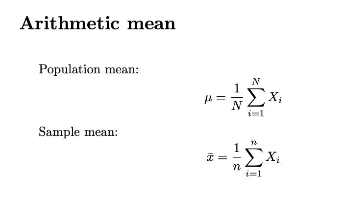
Next, let’s consider another familiar acquaintance, the arithmetic mean.
Crucially, the arithmetic mean is a measure of central tendency rather than dispersion. I highlight the mean here for two reasons: first, it is a key building block for the measures of dispersion that we will turn to next; and second, the mean helps to illustrate the distinction between a population and a sample that will be important in the latter part of this piece.
So, let’s talk populations and samples. In statistical terms, a population is a well-defined set that includes all possible units or cases that meet the criteria for inclusion in the study. A sample, meanwhile, is a subset of the population that is used to draw inferences about the population as a whole.
To illustrate this distinction, imagine that we wish to determine the average height of all the students in a school of 1,000 students. The population in this case would be all 1,000 students in the school. If we were to measure the height of every student and take the arithmetic mean of their heights, that would give us our population mean.
Since it may be impractical to measure the height of every student in the school, we could decide to take a sample of students instead. The method of selecting such a sample merits a discussion in and of itself, but the desired outcome is to select a sample that is representative of the population from which we can infer and generalise the characteristics of the population. For instance, we could randomly select 30 students and measure their heights to estimate the average height of the entire student population. This would give us a sample mean.
The practical method of calculating the mean is identical for both the population mean (denoted by μ) and a sample mean, (denoted by x̅). In both cases the calculation is to sum (Σ) all the values in a population and divide that sum by the count of the total number of values in the population. The crucial distinction here is in the notation. The count of the values in the population is denoted as N, while the count of the values in a sample is denoted as n.
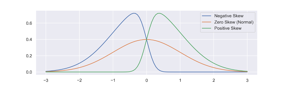
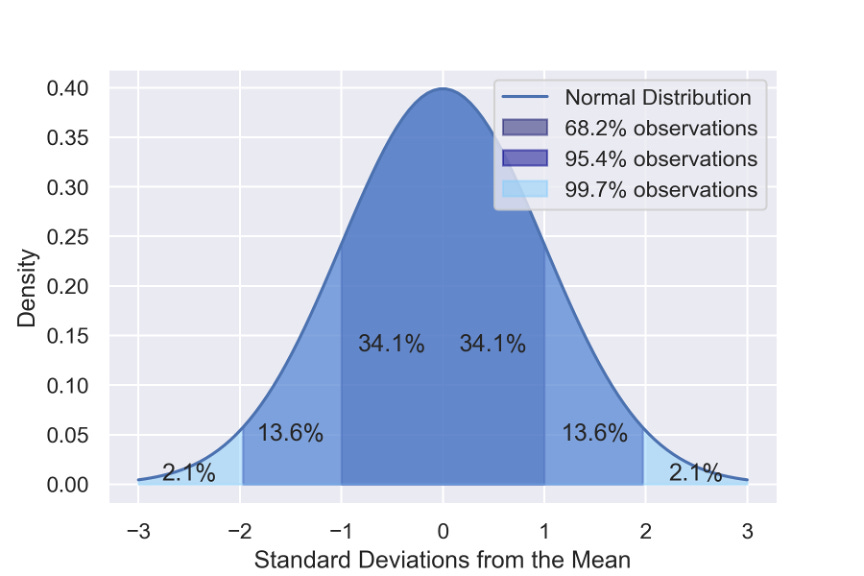
The mean is, in a statistical sense, efficient, since it takes into account all the available datapoints. But the mean is not without its imperfections. For instance, the less symmetrical and more skewed the data in the underlying dataset is, the less likely it is that the mean will provide an accurate statistical estimator. By contrast, if the distribution of the underlying dataset is closer to a ‘normal’ distribution, the mean is more likely to be an unbiased estimator. Mean is most effective for a normal distribution in which skewness (the measure of symmetry) = 0 and kurtosis (the measure of outliers) = 3.


To return to our measures of dispersion, let’s look at measures that use deviations in their calculation, starting with the sum of deviations from the mean. A deviation is the distance between a given data point and the mean. For any given population or sample, the sum of deviations from the mean is always equal to zero.

This is a fundamental flaw for any measure of dispersion, since it gives us the false impression that there is no variability at all in the data. Fortunately, There are two key ways to modify this measure of dispersion to avoid a zero result and produce an interpretable result.
The first option is to use the absolute deviations from the mean rather than simply using the deviations from the mean. An absolute deviation (denoted by |x|) treats any deviation from the mean the same regardless of its direction. In other words, -5 and 5 are treated identically. Mean absolute deviation (MAD), is a measure of dispersion that uses absolute values in this way, enabling us to generate a measure of dispersion that reveals the variability in the dataset visible.

Alternatively, we could square the numbers. Variance, uses this approach by squaring input values. Population variance is calculated as the summed differences between the squares of the mean and its data points, divided by the number of data points. Once again, this offers an interpretable result by ensuring that there is not zero result.
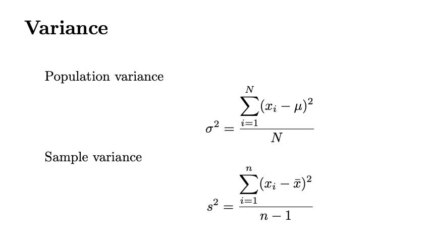
There are merits and demerits to using variance versus MAD. Variance is effective for comparing datasets with vastly different means since it measures the dispersion of the data relative to the mean. As in the prior example, however, variance is most effective when used on a dataset with a relatively normal distribution and less effective for datasets with outliers. This is because, where there are outliers, variance’s squaring approach gives added weight to those outlying values, bias-ing the final output. Mean absolute deviation, by contrast, is much less affected by outliers, so can more accurately reflect the variability of a dataset that contains distant values, or where the data is less normally distributed.
Additionally, variance lacks easy interpretability because it is derived from squared values so that the number it produces is not stated in the same units as the original data. Mean absolute deviation, on the other hand, retains the same units as the underlying data that it describes. Variance does, however, form the basis for the measure which I forewarned you about at the outset; standard deviation!
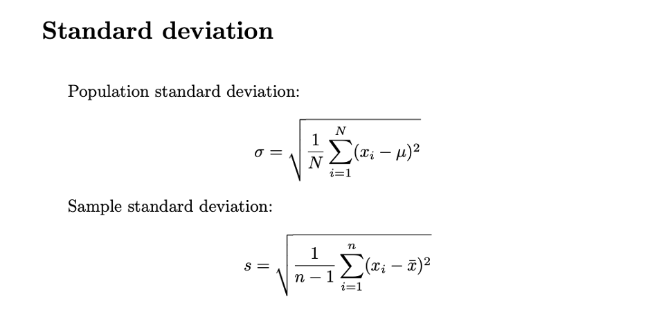
Standard deviation is calculated by taking the square root of the variance. A low standard deviation indicates that the underlying dataset tends to be closer to the mean, while a high standard deviation indicates that the values are more spread out.
To sum up, standard deviation, although most effective with normal populations, has become a widely-used measure of dispersion because it is highly interpretable, relatively efficient, and relatively unbiased compared to the other measures of dispersion that we have considered here.
Bessel’s Correction
To return to our distinction between populations and samples, there is an important additional twist needed when calculating standard deviation.
Calculating standard deviation for a population is as expected, we use our population arithmetic mean (μ) and the count of data points in the population denoted with an N.
The twist comes with the sample standard deviation. As we would expect, x̅ is used to denote the arithmetic mean and n is used to denote the count of the observations. The difference, however, comes in the denominator that divides the summed differences between the mean and its data points. It is not simply n, but rather n-1, otherwise known as Bessel’s Correction (named after the 18th-century Prussian mathematician who formalised the approach).
Any good stats textbook will inform us that this emendation is made in order ‘to correct for bias’. But what precisely is this bias that n-1 so deftly eradicates? Why does Bessel’s Correction produce a ‘less biased’ estimate of sample standard deviation? In short, what exactly does Bessel’s correction correct?
Understanding Bessel’s Correction
Let’s consider for a moment the very word statistic. A statistic refers to some piece of information derived from a sample (such as a mean, or standard deviation) which corresponds to some piece of analogous information about the population (again, such as mean, or standard deviation) which, in the case of the population, is called a parameter (rather than a statistic). Statistics are inherently hypothetical estimators that infer from smaller to larger.
We have now established very clearly that a sample is always a subset of a population - it does not actually represent the population, it merely attempts to represent the population. Having cemented our appreciation of that important difference, let’s now explore how sampling and ‘correcting’ our sampling affects the accuracy of our statistical measure.
For this exercise, I will be using a normal distribution. Here is an image of one million randomly-generated, normally-distributed points (generated using a sci-kit function). This will be our population:

I have visualised this population using a two-dimensional graph. This presentation style improves the interpretability of the data (and is more visually effective). For the purposes of our analysis, however, we only need to use the randomly-generated x-values. In other words, the data that is relevant could simply be visualised on a number line.

Since this is a population, we denote the observations with N. Here, N = 1,000,000 and, since the observations are normally distributed, we know that the mean of the data is 0.0, and the standard deviation is 1.0.
Let’s take two random samples, the first only 10 points and the second 100 points:

Taking both these samples and our original population, we can now calculate the standard deviation of each, with and without Bessel’s Correction (supposedly unbiased and biased, respectively):

Pleasingly, we can see that, at least in the case of this particular set of randomly-generated values, Bessel’s correction does improve the accuracy of our sample statistics.
We are looking for a SD of 1.0. Without Bessel, our 100-point sample is 0.043 away from the true value, with Bessel this is reduced to 0.038. Notably, the effect is even more pronounced when our sample size is smaller. The 10-point sample without Bessel’s correction is 0.072 away versus only 0.022 for the corrected version.
Interestingly, all our estimates are lower than the population standard deviation and increasingly lower for the smaller sample size. This is because unrepresentative points (‘biased’ points, i.e. points farther from the mean) will have more of an impact on the calculation of variance in smaller samples. Because the difference between each data point and the sample mean is being squared, the range of possible differences will be smaller than the real range if the population mean was used. To put it the other way, the larger your sample, the more of an opportunity you have to run into more points that are representative of the population (i.e. points that are close to the mean).
So Bessel’s Correction appears to work!
But does it always work? In short, yes and no. Bessel’s Correction is always a less biased estimator, however, it may return a result than is further from the true population mean than an uncorrected estimator.
In the below example (in the same Jupyter notebook), I have simply changed the random seed until I found a sample whose standard deviation was already close to the population standard deviation, and where n-1 was further from the actual figure.

To draw this piece to a close, we might conclude that Bessel’s Correction (dividing by n-1) always reduces bias but, because the potential sample-variances are themselves t-distributed, we will unwittingly run into cases where n-1 will overshoot the real population standard deviation.
That, I suppose, is the nature of statistics. We do not usually know the population values but we must make do with the information at hand. In the case of sample standard deviation, n-1 appears to be the most consistent tool we have to correct for bias.
Bibliography
Actual Proof: Gregory Gunderson Bessel
Dataset: Randomised values generated via Python and SciKit-Learn (make_gaussian_quantiles)
LaTeX Documentation: Overleaf
Python Documentation: Python Standard Library; Pandas; NumPy; MatPlotLib; Seaborn; Scikit-Learn
The latter part of this piece was directly inspired by The Reasoning Behind Bessel’s Correction